Capture your complex relational model in Cassandra
Source Code: https://bitbucket.org/johnmpage/gift/src/main/
Alignment of Concerns
The Cassandra database achieves scale by distributing data across multiple nodes. These nodes can be located on physically distant servers. This distributed architecture comes at a cost however; fast, efficient queries are best achieved by limiting the number of servers consulted when responding to data requests. Naturally a query that needs to consult a single server or node will be the most efficient. Every table in Cassandra supports multiple keys. The key designated as the “partition” key on a Cassandra table determines which node a row of data is stored on.
If we can organize our data model around the partition key, we can ensure data is returned quickly and efficiently. Gift seeks to simplify this process and enable a complex data model to be possible through a simple set of data annotations.
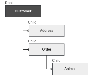
One constraint is placed upon the model to achieve an efficient retrieval of your relational data from Cassandra. A “root” data object must carefully chosen to organize the data model. Beneath this root object a data model of surprisingly complexity can be supported and queried efficiently.
Gift makes this simple. It automatically maps a relational schema into your Cassandra database, using several Hibernate-like annotations. The developer has only to generate a set of data classes that implement the data model. Once the relationship between the classes have the appropriate annotations added to the class definitions, Gift can automatically assemble the object tree including nested many-to-one from the results of a Cassandra query language (CQL) query.
Single Table Schema
How does Gift accomplish this? Cassandra does NOT supporting JOINs between tables, the typical means of mapping out one-to-many relationships, a feature of relational database. Cassandra does support multiple indexed keys. Gift leverages multiple keys and the efficient storage of null values.
Storing multiple data types in a single table, we leverage the capability to support a large number of row indexes. One dedicated column uniquely identifies row types, while the other indexed columns act as foreign keys to provide an association between individual rows. These keys can be empty if there is no relationship. The only required column is the key associating the row with the root entity.
How does the data in the table look? Below we see an example of a hypothetical dataset for a pet store. Because this dataset supports a Customer based interface, every row includes key that associate the row with a particular Customer. In this simplified example, we can see that Customer Smith has one address in Boston. Order 123 is associated with Customer Smith and includes one Cat.
| Customer Id | Address Id | Order Id | Animal Id | Data Type | Last Name | City | Order No | Type |
|---|---|---|---|---|---|---|---|---|
| cus1 | Customer | Smith | ||||||
| cus1 | add1 | Address | Boston | |||||
| cus1 | ord1 | Order | 123 | |||||
| cus1 | ord1 | ani1 | Animal | Cat |
The secondary indexes act not as unique identifiers for data types as well as foreign keys, mapping relationships between entities.
The only restriction is that every row must be a child of the root entity.
Usage
Gift provides a simple way to build a relational data model. In order to generate the pet store model described above, creates four data classes:
The Customer class can be defined as follows:
import net.johnpage.cassandra.gift.annotations.*;

@Root
public class Customer {
    public Customer(){}
    @Id
    @ClusterKey
    @Column(value = "cstId")
    public String customerId;
    @Column(value = "cstlastname")
    public String lastname="";
}
The @Root annotation establishes this class as the root class of data. The key for this data type is designated by the @Id annotation. The Cassandra column name is specified with the @Column annotation. In this example we chose to use a three letter prefix “cst” in front of all the columns associated with the Customer. The last name column is defined as “cstlastname“.
We define the first child of the Customer entity by first adding the child as a property of Customer.
@Root
public class Customer {
    public Customer(){}
    @Id
    @ClusterKey
    @Column(value = "cstId")
    public String customerId;
    @Column(value = "cstlastname")
    public String lastname="";
    @ChildCollection(childClass = Order.class)
    public List<Order> orderList = new LinkedList<>();
}

The Order class is as follows:

public class Order {
    public Order(){}
    @Id
    @ClusterKey
    @Column(value = "ordId")
    public String orderId;
    @Column(value = "cstid")
    @ParentKey(parentClass = Customer.class)
    public String customerId;
}

Here the unique id for Orders is annotated with @Id. Every class needs to identify the root class that they are associated with it. In Order, we add the "customerId" to maintain the relationship to the root class.  "orderId" provides a unique identifier for the class.
This child of Customer can in turn have children of it’s own. Here we define a list of Animals for example:
@ChildCollection(childClass = Animal.class)
public List<Animal> animalList = new LinkedList<>()
The Animal class is defined as follow:
public class Animal {

    public Animal(){}

    @Id
    @ClusterKey
    @Column(value="anmid")
    public String animalId;

    @ParentKey(parentClass = Order.class)
    @Column(value = "ordid")
    public String orderId;
}
Once your dataset has been assembled in your business code, it can be saved and/or updated with a a single line of code:
CassandraClient.insert(customer);To query the database, a single line will suffice:
String query = "SELECT * FROM customer where clsid='c1'";
Customer this customer = CassandraClient.query(query, Customer.getClass())
Currently some knowledge of the schema is required to query the database, but a simple query like the one before quickly returns the complete Customer record for one customer, including their Address and all of their Orders.
Because the root I’d also servers as the Partition Key, the query only visits one node and the query is fast and efficient. The framework handle all the keys seamlessly under the hood. The developer can begin using the Customer immediately after running the query.

